The least squares problem shows that the series of equations
\tilde{y}_{m \times 1} = H_{m \times n} \cdot \hat{x}_{n \times 1}
mapping H inputs to y measurements using x model parameters has the analytical solution
\hat{x}_{n \times 1} = \left(H ^T H \right )^{-1}_{n \times n} H^T_{n \times m} \cdot \tilde{y}_{m \times 1}
We did this by defining the residual as
r_{m \times 1} = \underbrace{\tilde{y}}_{\text{measured}}-\underbrace{\hat{y}}_{\text{estimated}} = \tilde{y}_{m \times 1} - H_{m \times n} \cdot \hat{x}_{n \times 1}
And minimizing the residual sum squared.
J_{1 \times 1} = \frac{1}{2} \cdot \left( r^T_{1 \times m} \cdot r_{m \times 1} \right)
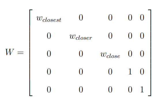
Now we look to apply a weighting matrix (with non-zero values along the diagonal) to emphasize or de-emphasize the certain calculated residuals.
W_{m \times m} = \begin{bmatrix}
w_0 & 0 & 0 & 0\\
0 & w_1 & 0 & 0\\
0 & 0 & \ddots & 0 \\
0 & 0 & 0 & w_{m-1}
\end{bmatrix}
such that the residual sum squared becomes
J_{1 \times 1} = \frac{1}{2} \cdot \left( r^T_{1 \times m} \cdot W_{m \times m} \cdot r_{m \times 1} \right)
To minimize the residual sum squared, we need to find where the derivative is zero.
This time we're going to use the chain rule to do it
\frac {\partial J}{\partial x}_{1 \times n} = \frac {\partial J}{\partial r}_{1 \times m} \frac {\partial r}{\partial x}_{m \times n}
\frac {\partial J}{\partial r} =
\frac{1}{2} \cdot\frac {\partial }{\partial r} \left( r^T_{1 \times m} \cdot W_{m \times m} \cdot r_{m \times 1} \right) =
\frac{1}{2} \cdot r^T_{1 \times m} \cdot \left( W_{m \times m} + W^T_{m \times m} \right)
and
\frac {\partial r}{\partial x} =
\frac {\partial }{\partial x} \left( \tilde{y}_{m \times 1} - H_{m \times n} \cdot \hat{x}_{n \times 1} \right) =
- H_{m \times n}
Such that
\frac {\partial J}{\partial r}_{1 \times m} \frac {\partial r}{\partial x}_{m \times n} =
\left( \frac{1}{2} \cdot r^T_{1 \times m} \cdot \left( W_{m \times m} + W^T_{m \times m} \right) \right)_{1 \times m} \cdot \left( - H_{m \times n} \right)
Which combined becomes
\frac {\partial J}{\partial r} \frac {\partial r}{\partial x} =
- \frac{1}{2} \cdot\left( r^T_{1 \times m} \cdot \left(W_{m \times m} + W^T_{m \times m}\right) \cdot H_{m \times n} \right)
And substituting back in...
\frac {\partial J}{\partial x} =
- \frac{1}{2} \cdot\left( \left(\tilde{y}_{m \times 1} - H_{m \times n} \cdot \hat{x}_{n \times 1} \right )^T_{1 \times m} \cdot \left(W_{m \times m} + W^T_{m \times m}\right) \cdot H_{m \times n} \right)
Applying the transpose rules
\frac {\partial J}{\partial x} =
- \frac{1}{2} \cdot\left( \left(\tilde{y}^T_{1 \times m} - \hat{x}^T_{1 \times n} \cdot H^T_{n \times m} \right )_{1 \times m} \cdot \left(W_{m \times m} + W^T_{m \times m}\right) \cdot H_{m \times n} \right)
And clean up the negative sign
\frac {\partial J}{\partial x} =
\frac{1}{2} \cdot \left( \hat{x}^T_{1 \times n} \cdot H^T_{n \times m} - \tilde{y}^T_{1 \times m} \right )_{1 \times m} \cdot \left(W_{m \times m} + W^T_{m \times m}\right) \cdot H_{m \times n}
Such that we can assume the derivative to be 0 and build the equation
\hat{x}^T_{1 \times n} \cdot H^T_{n \times m} \cdot \left(W + W^T\right) \cdot H_{m \times n} = \tilde{y}^T_{1 \times m} \cdot \left(W + W^T\right) \cdot H_{m \times n}
Taking the transpose of both sides preserves equality
H^T_{n \times m} \cdot \left(W^T + W\right) \cdot H_{m \times n} \cdot \hat{x}_{n \times 1} = H^T_{n \times m} \cdot \left(W^T + W\right) \cdot \tilde{y}_{m \times 1}
And finally we can solve for the x parameters.
\hat{x}_{n \times 1} = \left( H^T \cdot \left(W^T + W\right) \cdot H \right )^{-1}_{n \times n} \cdot H^T_{n \times m} \cdot \left(W^T + W\right) \cdot \tilde{y}_{m \times 1}
If W indeed only has elements along its diagonal
\hat{x}_{n \times 1} = \frac{1}{2} \left( H^T \cdot W \cdot H \right )^{-1}_{n \times n} \cdot H^T_{n \times m} \cdot \left(2 \cdot W\right) \cdot \tilde{y}_{m \times 1}
And simplifies to
\hat{x}_{n \times 1} = \left( H^T \cdot W \cdot H \right )^{-1}_{n \times n} \cdot H^T_{n \times m} \cdot W \cdot \tilde{y}_{m \times 1}
